While working with Microsoft Excel you will come across certain scenarios where you will have to retrieve a specific Cell Entry from a large data set. And to do so, you will need to learn how to use VLookup Function in Excel.
![]()
So what is VLookup? Microsoft Excel comes with hundreds of built-in formulas and VLookup is one of them. As you might have guessed the ‘V’ in VLookup stands for Vertical. This means you can search for a certain entry across a certain Column in Excel.
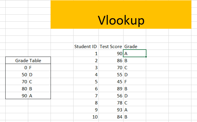
But how does it work and where can you use this formula? Let’s start by answering the later one. See the data set below.
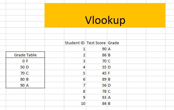
On the right, I have a Grade Table which holds what number a student must get to be assigned a certain grade. For example, if students get 90 or 90+, they will get the Grade A. Most schools will have this grading table built long before exams start. And they might apply to multiple classes. So this means we cannot make any changes to the Grade Table.
Now suppose at the end of the first quiz, the results are out. And now all you have to do is assign a Grade to the scores. In such a scenario you can retrieve values from the pre-specified Grade Table right beside the individual test scores using the VLookup function.
Now let’s answer the second question, how to use the VLookup Function.
How To Use VLookup Function In Excel
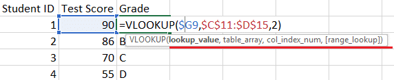
Now, for beginners, you only need to specify three arguments for the formula- Lookup Value, Table Array, and Col Index Number.
You can either apply this formula individually to every cell under the column Grade. Or you can Lock cells inside the formula and get Grades for all the 10 cells with one single keyboard press. We are going to learn just that!
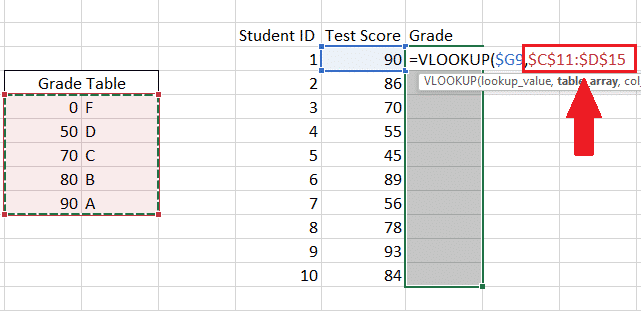
In the second argument Lookup Value, you need to Lock the Column ‘G’ which holds all the Test Score Values. And secondly, you need to lock the entire table in the second argument Table Array. We are going to learn how to lock cells in Steps Four and Five.
First Step: Select all the cells under the Grades Column.
Second Step: Press the ‘=’ button on your keyboard and write VLookup.

Third Step: Hit Tab when the VLookup function is highlighted.
Fourth Step: For the first argument, select the first row under Test Score Column. And put a Dollar Sign in front of ‘G’. You can also press the F4 key three times to put a dollar sign in front of a Column.
Fifth Step: Select the Grade Table as the Table Array and Lock it completely. This means you are putting dollar signs in front of both the row and column. You can press the F4 key just once to do it.
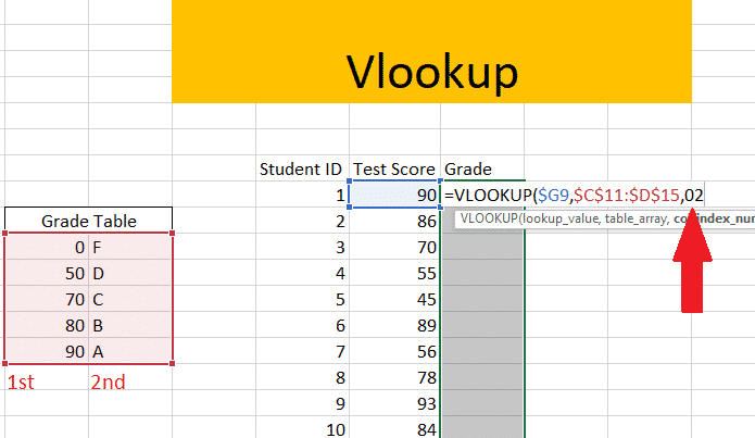
Sixth Step: Give the Column Index. The Actual Grades are sitting on the second column of the Grade Table. This is why simply writing ‘2’ would do the work.
Seventh Step: Now Hit Ctrl+Enter.
Wrapping Up!
If you face any trouble getting it right make sure you are following the instructions correctly. Or simply leave a comment below and we will get back to you.
Also, let us know what other practical applications of VLookup function you would use to cover. In the meantime here is a quick blog on how to freeze cells in Excel.

![Read more about the article [Tutorial] How To Repair Windows 7 Boot](https://thetechjournal.com/wp-content/uploads/2012/02/starting-windows-7-512x284.jpg)
![Read more about the article [Tutorial] How To Jailbreak Your iPad on iOS 5.1.1 Using Absinthe 2.0 – Windows](https://thetechjournal.com/wp-content/uploads/2013/01/Using-Absinthe-2.0-1.jpg)