Do you have to work with Microsoft Excel on a regular basis, or are you just an Excel enthusiast? Know that, you will face situations where you will have to work with huge sets of data. And in those cases, seeking help from slick Excel tricks will save your valuable time and effort.

If you have a huge data set, you might want to lock the header cells containing the credentials of the data table. Usually, you will have the credentials at the top row of your data set. Also, it is very likely that you will have to include credentials of your data set across the first few columns.
How To Freeze Cells In Excel
Microsoft Excel includes a very handy tool that keeps certain rows or columns visible as you scroll up-down or left-right. Now let’s see two hypothetical examples and learn the use of this life-saving feature.
Lock Multiple Rows
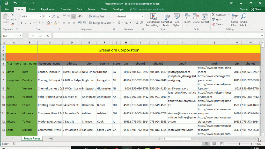
Let’s break down the instructions. In the below screenshot, you can see I have merged the 1st, 2nd, and 3rd, 4th rows together. So, now I want to freeze the first 4 rows.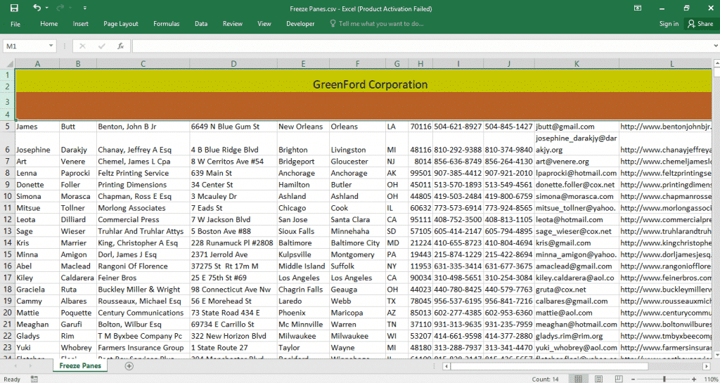
In order to do so, I have to select the 5th row. Hover your mouse over the rightmost corner of the spreadsheet and click on row 5. After you have clicked on the 5th row, it will be highlighted in a dim blue color. Now, Head over to View>Freeze panes and pick the first option-Freeze Panes.
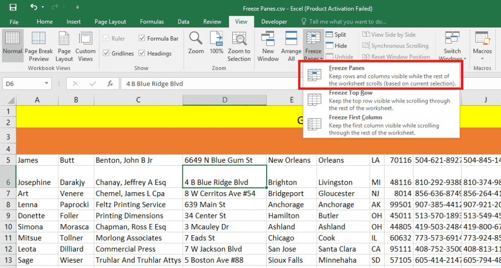
You are all good to go. Now use the mouse to scroll down and you will see the first 4 rows have been locked.

Freeze Multiple Columns
In the screenshot below, you can see the first two columns are highlighted in green. Now, let’s freeze these two columns.
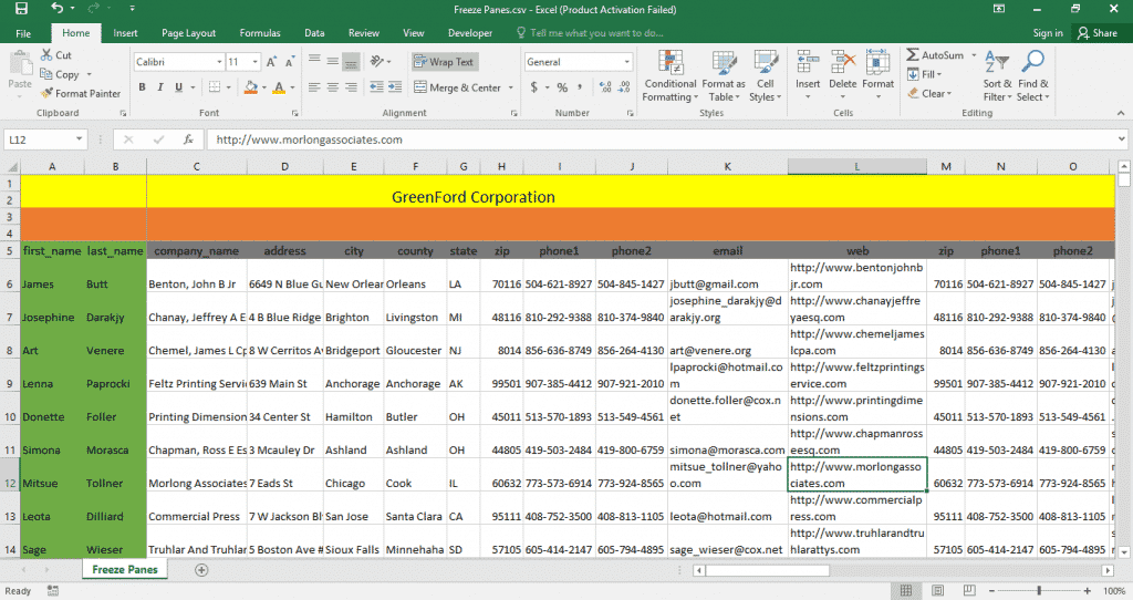
In order to freeze the 1st and 2nd columns, I need to select the 3rd column and navigate to View>Freeze Panes. Hover your mouse over the 3rd column and right click on it. Now head over to View>Freeze Panes.
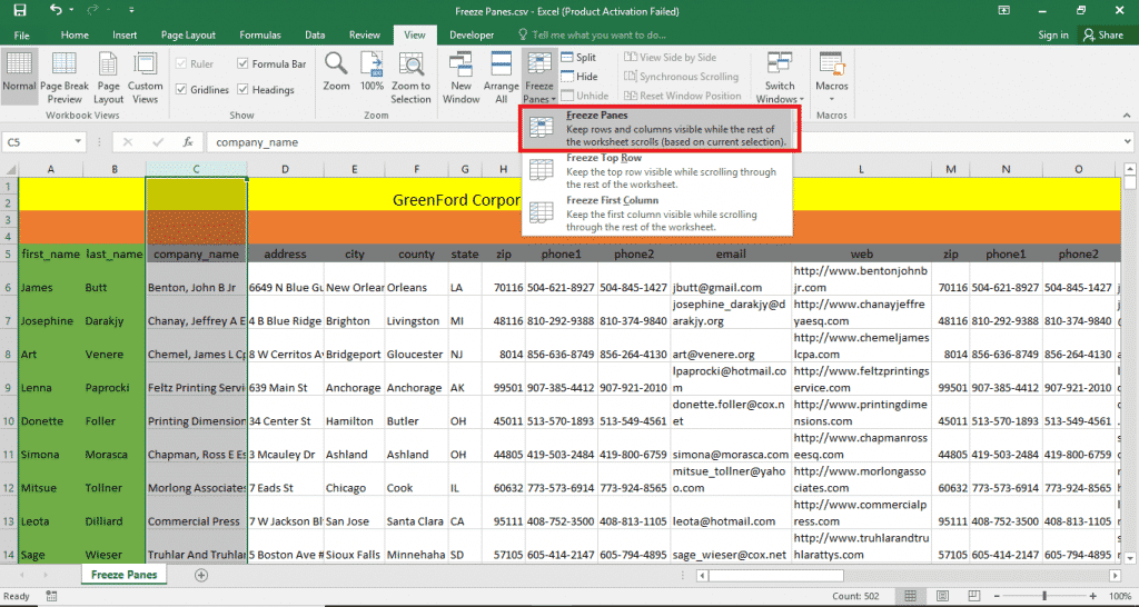
From the drop-down select Freeze Panes. That’s it! Now use your mouse to scroll horizontally across the spreadsheet.
Wrapping Up!
Want to learn more Microsoft Excel tricks? Here is a quick blog that will teach you how to add legends in Excel Charts.



![Read more about the article [Tutorial] How To Move Contents From Android To iPhone](https://thetechjournal.com/wp-content/uploads/2014/09/Switching-From-Android-To-iPhone-512x256.jpg)
close in weapons system [url=https://otvetnow.ru]https://otvetnow.ru[/url] test tablet